

Modelling Actors with Redex: Part III
Mon 3 Aug 2026 15:10 CEST

This is the third part of a series of three articles on modelling actor-like systems1 2 using PLT Redex.
(The first sketch of this part of the series was written in August 2016, a day after the other two. Ten years later, I’m finally getting around to finishing it off!)
- Part I: The Functional Fragment: ISWIM in Redex
- Part II: The Communicating Fragment: Actors in Redex
- Part III: Efficiency vs. Nondeterminism
 Like the previous posts, this post is written as a literate
Racket source file, and is licensed CC-BY
4.0. You can
download it and run it yourself.
Like the previous posts, this post is written as a literate
Racket source file, and is licensed CC-BY
4.0. You can
download it and run it yourself.
Efficiency vs. Nondeterminism
At the end of Part II, we had a working model of Actors that could handle only small example programs because of the enormous number of possible interleavings the naive approach to scheduling generated.
In this post, we will take advantage of the fact that certain interleavings cannot be distinguished by actors. By cutting back on such unobservable nondeterminism, we end up with a model which yields not only smaller, more legible traces, but also gives dramatically improved Redex runtimes. The speed-up allows our model to scale much further without going to a completely sequential setting.
Running Example: A Two-Actor Race
Let’s take the following term as our running example. The
primordial actor first retrieves its own process ID using
(self), storing it in a local variable w, and then
spawns two actors which race to send different messages
to w. The primordial actor receives the first message to
arrive, and yields it as its final value, leaving the other
message unread in its mailbox:
(let ((w (self)))
  (spawn (send w 1))
  (spawn (send w 2))
  (receive))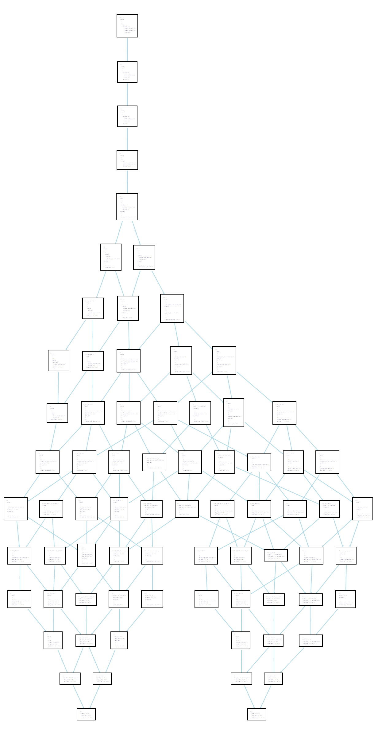
Figure 1: Ultra-fine-grained trace, 74 distinct states, 15-step paths.
Evaluating this program using the model of Part II exposes
extremely fine-grained interleavings of reductions, almost all of
which are not observable by any actor. Figure 1 is a screen capture of
the resulting traces as rendered by Redex, with the starting state at
the top and the two final states at the bottom.3
We see 74 densely-interconnected distinct states, with each path having
15 steps, even though there are only about 6 “interesting” moments in
the execution of the program, and only two possible final outcomes.
Redex computes this trace in approximately 1015ms (best of 3) on my
Apple M3 Pro system.
Interleavings Form Equivalence Classes
The way our send and deliver reduction rules interact
gives our configurations an unbounded queue of messages “in
the network” on their way from their sender to their
receiver.
Because send and deliver are chosen independently, this
gives multiple distinct reduction sequences when any two
messages are “in flight” at the same time.
In our example, two actors simultaneously send a message to
the primordial actor: (send w 1) and (send w 2). All of
the following reduction sequences are possible:
send1,deliver1,send2,deliver2send1,send2,deliver1,deliver2send1,send2,deliver2,deliver1send2,deliver2,send1,deliver1send2,send1,deliver2,deliver1send2,send1,deliver1,deliver2
Even though we, looking at the global trace from the outside,
can see such differences, there is no possible way that w
can ever detect them. The receiving actor will only ever see
1 before 2 or 2 before 1.
That is, the contextual observational equivalence available to us is much coarser than the equivalence over the traces generated by our reduction relation. Unless we are interested in modelling fine detail of how a message propagates across the network connecting our actors, the comparative coarseness of our observational equivalence justifies omitting this level of detail.
One approach to doing so is to alter all our configuration-level rules
to treat the configuration’s queue as a one-place buffer, and to
require that the buffer be empty in every rule except send,
deliver, and failed-delivery.
That is, most of our reduction rules will now have the general form
(--> (() (actor_0 ... (pid : mailbox_0 expr_0) actor_1 ...))
     (() (actor_0 ... (pid : mailbox_1 expr_1) actor_1 ...)))
constraining the configuration’s queue to be empty.
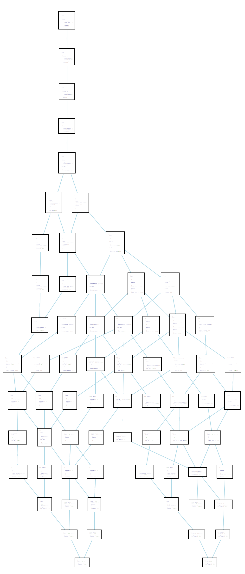
Figure 2: Very fine-grained trace, 68 distinct states, 15-step paths.
The file det0b.rkt contains the complete model after making these changes. Evaluating our example program now results in the trace of Figure 2. We have reduced the number of distinct states from 74 to 68, though the total path length is still 15. Programs with more messages “in flight” at the same time will see more dramatic improvements from this alteration to the model. Even though the number of states is only modestly smaller, we have already achieved a dramatic improvement in runtime: Redex computes this trace in approximately 178ms, which is almost six times faster than the model we started from.
We have improved the way we use our configuration’s queue, but we’re not quite done with it yet; before we revisit it, however, we will investigate splitting intra-actor reductions from inter-actor reductions.
Intra-Actor Reductions Cannot Be Observed
The coarseness of our observational equivalence justifies omission of even more detail. Consider the evolution of the following ISWIM term:4
(+ 1 (+ 2 (+ 3 4))) ──delta──>
(+ 1 (+ 2 7      )) ──delta──>
(+ 1 9            ) ──delta──>
10
At no point does the reduction sequence do anything that a neighbouring actor could observe, and at no point does it observe anything that a neighbour might have been doing.
It is only when actors perform side effects such as (send
...) or (receive) or (spawn ...) that specific
interleavings become distinguishable by other actors in the
system.5
Our goal, then, is to stop Redex from considering all these indistinguishable interleavings, leaving only the interleavings involving side effects. The result will be another reduction in inessential nondeterminism.
To do this, we split the plain ISWIM notions of reduction out
into a separate reduction relation, ISWIM+Actors-inner-red,
that is literally exactly the same text as ISWIM-red in
redex-iswim.rkt except with ISWIM+Actors as
the underlying language instead of plain ISWIM:
(define ISWIM+Actors-inner-red
  (reduction-relation ISWIM+Actors
    ;; ... beta, delta rules etc. omitted.
    ;;     They are exactly the same as in redex-iswim.rkt.
    ))
We remove the plain ISWIM “==>” shortcut rules (that now
live in ISWIM+Actors-inner-red) from our main
ISWIM+Actors-red reduction relation, and replace them with
a single rule that invokes ISWIM+Actors-inner-red at least
once and as many times as possible:
(==>* expr_0 expr_2
      (where (expr_1a ... expr_1 expr_1b ...)
             ,(apply-reduction-relation ISWIM+Actors-inner-red
                                        (term expr_0)))
      (where (expr_2a ... expr_2 expr_2b ...)
             ,(apply-reduction-relation* ISWIM+Actors-inner-red
                                         (term expr_1))))
with
[(--> (() (actor_0 ... (pid : mailbox A) actor_1 ...))
      (() (actor_0 ... (pid : mailbox B) actor_1 ...)))
 (==>* A B)]
This is a lot to unpack! It reads like this:
- An actor may take a
-->-step if the actor’s expression can take a==>*-step (Lines 9–11). - An expression
expr_0takes a==>*-step to someexpr_2if:- there exists some
expr_1such thatexpr_0can step toexpr_1viaISWIM+Actors-inner-red(Lines 2–4), and expr_1can step toexpr_2via zero or more repetitions ofISWIM+Actors-inner-red(Lines 5–7).
- there exists some
One complication is that the rule here relies on Redex’s mechanism for
escaping into unrestricted Racket, written with a prefix comma: the
“,” on lines 3 and 6 precedes calls to the Racket functions
apply-reduction-relation and apply-reduction-relation*, which live
in a different namespace to our language’s syntax and our defined
metafunctions.
Another complication is that we’re using the awkward-looking (x_0a
... x_0 x_0b ...) idiom for nondeterministic selection of a
term from a list of terms, first introduced in Part II. Redex will match zero or more
“x_0a”s before binding a unique “x_0” and then again matching
zero or more “x_0b”s. Because in general there are many ways of
doing this, the result is inclusion of all the possibilities as
potential reduction steps.
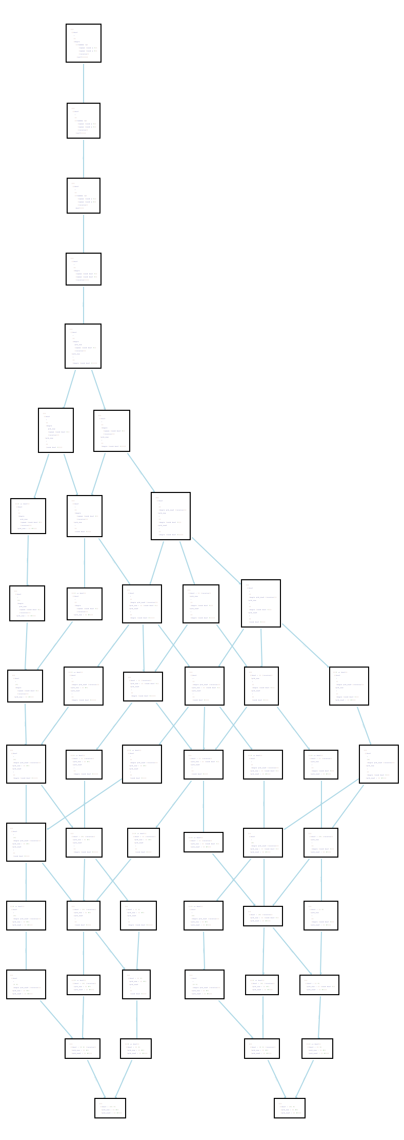
Figure 3: Fine-grained trace, 52 distinct states, 14-step paths.
The file det1.rkt contains the complete model after making these
changes. Evaluating our example program now results in the trace of
Figure 3. We have reduced the number of distinct states from 68 to 52,
and the total path length is now 14, one step shorter because two steps
merge as a consequence of the “greedy” nature of
apply-reduction-relation*.
This doesn’t seem too impressive, but remember our example has very little actor-local computation. Programs with more such computation will see much more dramatic reductions in the number of unobservable intermediate states. And again, even though the number of states is not much smaller, the computation time has improved: Redex computes this trace in about 61ms, roughly 3× faster than the previous version and around 16× faster than the unchanged model of Part II.
This Only Works For Non-Diverging Programs
There’s an important caveat that has to be discussed at this point.
If we can guarantee that all individual actors in our system are
non-diverging, then this approach is fine. A non-diverging actor
always takes a finite number of reductions to either yield a final
value or engage in an effect such as self, send, receive or
spawn.
A diverging actor is one that reduces internally “forever”.
For example, an actor running the expression ((rec loop
(lambda () (loop)))) produces an infinite chain of repeating
unfold, beta, begin-one steps:
 ╭─────────────> ((rec loop (lambda () (loop))))
 │                  ╷
 │                  │ unfold
 │                  V
 │   ((lambda () ((rec loop (lambda () (loop))))))
 │                  ╷
 │                  │ beta
 │                  V
 │        (begin ((rec loop (lambda () (loop)))))
 │                  ╷
 ╰──────────────────╯
      begin-one
If we try to use our current model to explore a diverging
actor, Redex itself will get stuck. By appealing to the
possibly-nonterminating Racket procedure
apply-reduction-relation* as part of ISWIM+Actors-red, we
lose the nice progress property Redex offers us.
If you wish to work with a system that permits diverging
actors, there are various more-or-less unsatisfactory ad-hoc
remedies you could try: for example, you could define an
apply-reduction-relation/n that takes a step count n and
yields the term after at most n steps. The drawback is that
your system will include spurious interleavings every time the
limit n is actually reached by some actor.
For most purposes, though, it seems to me that the requirement for non-diverging actors is fairly modest. We will assume it for the remainder of this post.
Combining Effects and Internal Reductions
As it stands, our ISWIM+Actors-red relation still takes a separate
step to perform one or more internal ISWIM+Actors-inner-red
reductions. But the very possibility of internal reductions only arises
as the result of some effect: internal reductions in an actor can only
be possible (a) immediately after it is spawned, or (b) immediately
after the completion of some effect it has requested.
This suggests the idea of combining effectful
ISWIM+Actors-red reductions with computational
ISWIM+Actors-inner-red reductions, and removing the need
for the shortcut ==>* steps entirely.
Because plain ISWIM is deterministic (see exercise 4 in Part I),
there’s an elegant way to do this in Redex. We know that
apply-reduction-relation* will always produce a list containing
exactly one term, as a consequence of ISWIM’s determinism. We remove
the ==>* arrow and the with clause from ISWIM+Actors-red
entirely, and instead adjust our effect-handling rules to invoke a new
metafunction reduce-inner:
(define-metafunction ISWIM+Actors
  reduce-inner : expr -> expr
  [(reduce-inner expr)
   ,(first (apply-reduction-relation* ISWIM+Actors-inner-red
                                      (term expr)
                                      #:error-on-multiple? #t))])
For example, here’s the modified self rule:
(--> (() (actor_0 ... (pid : mailbox (in-hole context (self)))             actor_1 ...))
     (() (actor_0 ... (pid : mailbox (reduce-inner (in-hole context pid))) actor_1 ...))
     self)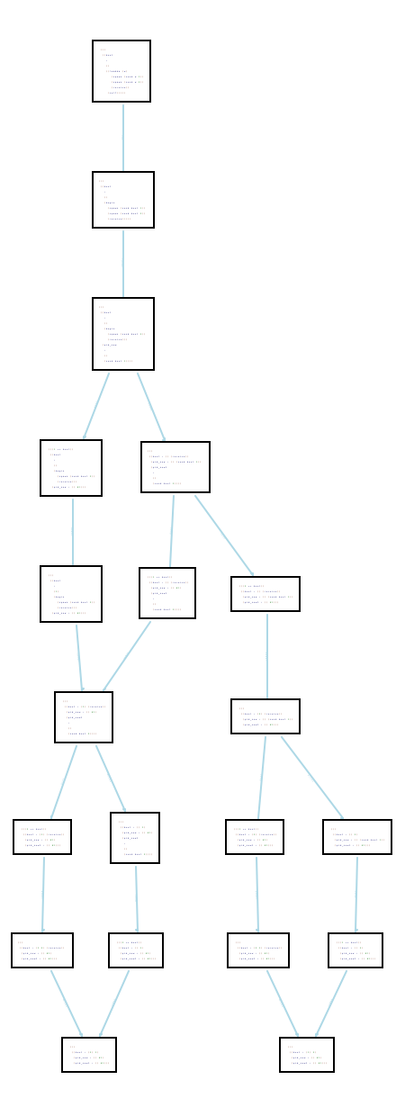
Figure 4: Reasonable trace, 20 distinct states, 8-step paths.
The file det1b.rkt contains the complete model at this stage. With these changes applied, our example program now produces the trace of Figure 4. We have a much more reasonable 20 states, now, and the paths are only 8 steps long. The computation time is dramatically better than before: Redex completes the trace in only 2ms, hundreds of times faster than the model of Part II.
Looking at the branching pattern of the trace graph, we see
branching exactly where we expect “interesting”
nondeterminism: the second spawn and second send race
with the first send, and the final receive races with
whichever of the sends is last to be delivered.
The strategy of “hiding” intra-actor reductions as part of inter-actor effect handling has dramatically simplified our traces. For a final touch, we will revisit our treatment of the configuration’s queue, which we made into a one-place buffer as our first improvement above.
Broadcasting sends With No Queue At All
ISWIM+Actors-red still separates the send rule, which places an
in-flight message into the configuration’s queue, from the deliver
rule, which consumes from the queue and places each message in its
target actor’s mailbox. This, combined with the “empty queue”
restriction on all the other rules, results in a regular two-step
pattern seen whenever a send is available.
Combining send and deliver into a single rule, delivering messages
directly into their target mailbox, gives us two benefits: we
eliminate the two-step pattern, and we simplify configurations. After
the change, a configuration is a simple list of actors without any
message queue at all.
This is the revised send rule:
(--> (actor_0 ...
      (pid_1 : mailbox (in-hole context (send pid value_0)))
      actor_1 ...)

     ((deliver pid value_0 actor_0) ...
      (deliver pid value_0 (pid_1 : mailbox (reduce-inner (in-hole context #t))))
      (deliver pid value_0 actor_1) ...)

     send)
The left hand side of the rule selects an actor ready to
perform a send. The right hand side broadcasts the sent
message to all actors in the configuration. The new
metafunction deliver enqueues the message only when the
pid of the receiving actor matches the pid to which the
message is addressed:
(define-metafunction ISWIM+Actors
  deliver : pid value actor -> actor

  [(deliver pid value (pid : (value_0 ...) expr))
   (pid : (value_0 ... value) expr)]

  [(deliver pid value actor)
   actor])
Because the definition of configuration has been simplified in the
ISWIM+Actors language, the other reduction rules in
ISWIM+Actors-red are correspondingly simplified.
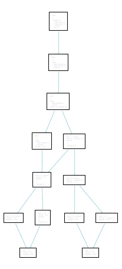
Figure 5: Good trace, 13 distinct states, 6-step paths.
The file det1c.rkt (and, indeed, this file itself) contains the code for this final variant of the model.
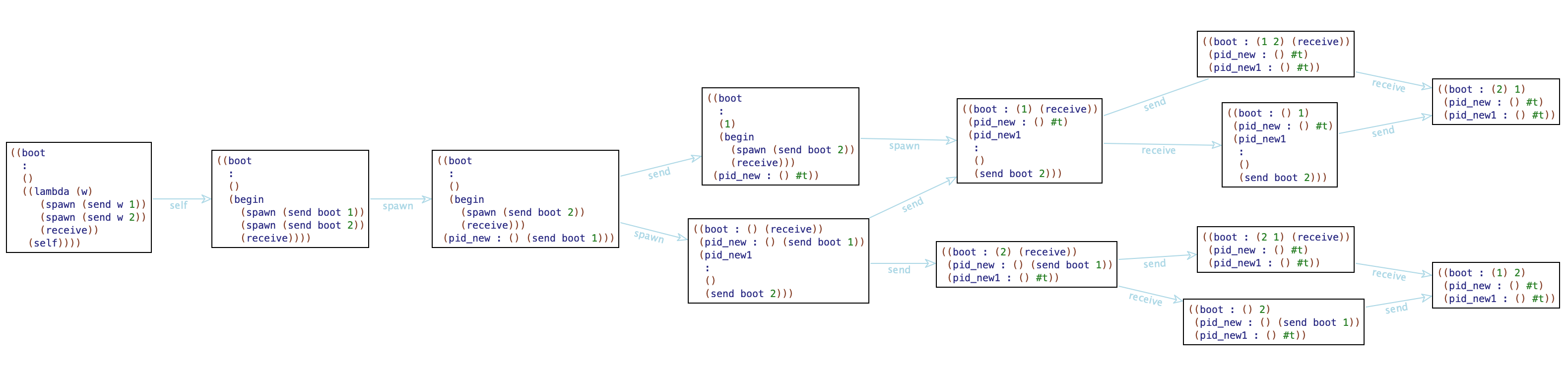
Combining the send, deliver and failed-delivery rules like this
results in the trace of Figure 5 for our example program. We see the
same branching pattern as in Figure 4, but every two-step
send/deliver pair has been replaced by a single send transition.
The time taken to compute the trace is roughly as it was in the
previous step, about 2ms. The resulting graph has only 13 distinct
states, and each path is exactly 6 steps long, matching the number of
“interesting” moments we expected originally.
In fact, it’s now possible to actually read and understand the trace. Here it is, rendered with a more legible font size, and left-to-right instead of top-to-bottom (click the image to embiggen):
Conclusion
The following table summarises the progress we have made with respect to evaluation of our running example program:
| Variant | States | Path length | Time to compute | Approx. speedup |
|---|---|---|---|---|
| Part II | 74 | 15 | 1015 ms | 1× |
| One-place buffer | 68 | 15 | 178 ms | 5.7× |
| Embedded ISWIM steps | 52 | 14 | 61 ms | 16.7× |
| Merged ISWIM steps | 20 | 8 | 2 ms | 500× |
One-step send |
13 | 6 | 2 ms | 500× |
We started this process with the model of Part II, which had a single reduction relation with 6 communication-related rules and 7 computation-related rules. It generated overly-detailed traces that admitted many uninteresting interleavings, and Redex took more than a second on my system to evaluate our example program.
We ended with two layered reduction relations: one “inner” relation, exactly that of plain ISWIM, having the 7 computation-related rules, and a separate “outer” communication-oriented relation with exactly 4 rules, one for each kind of effect available to an actor. It generates traces that are much closer to the observational power of actors themselves, and Redex takes only a couple of milliseconds to evaluate the example program, making our final model several hundred times faster than the one we started with.
At this point, we’ve reached the end of this series of posts on modelling actor-like systems in PLT Redex. I chose a “realistic” notion of observational equivalence as a place to stop. With the model as it stands, actors will (I claim!) observe all relevant interleavings of events. That is, there’s a useful notion of nondeterminism still embodied in the system.
In order to work with truly large (or diverging!) examples, however, depending on the aspect one is interested in,6 one might have to move to a fully deterministic system to allow Redex to operate efficiently enough to be useful. Such a system corresponds to a sequential (functional!) simulation of a concurrent system, and always picks some specific interleaving of events out of all possibilities. While chapter 4 of my dissertation gives an example of this kind of reduction system, we will leave the idea unexplored here for now, perhaps to be picked up in a future post.
Appendix: The Final Model, Piece By Piece
In the remainder of the post, I’ll present the final executable source code in its entirety.
Preliminaries
As before, we need the #lang header, and we require both Redex and
the base language definition ISWIM from Part I.
#lang racket
(require redex)
(require (only-in "redex-iswim.rkt" ISWIM))
Syntax
Just as in Part II, we extend the core ISWIM language with effects, process IDs, actors, and configurations.
(define-extended-language ISWIM+Actors ISWIM
  (expr ....
        (send expr expr)   ;; sends the second arg to the first arg, a PID
        (receive)          ;; blocks, waiting for the next message
        (self)             ;; evaluates to the PID of the calling actor
        (spawn expr ...))  ;; spawns a new actor which performs the exprs.

  (value ....
         pid)              ;; a process ID (PID) is a value

  (pid variable-not-otherwise-mentioned)  ;; we represent PIDs using names
Evaluation contexts must be extended to allow reduction in the PID and message positions of
a send.
  (context ....
           (send context expr)
           (send pid context))
Unlike Part II, our configurations are now mere lists of actors, and have no configuration-wide queue of messages “in the network”.
  (configuration (actor ...))
  (actor (pid : mailbox expr))
  (mailbox (value ...)))
Reduction Rules and Metafunctions
Also unlike the model of Part II, which embeds the plain ISWIM notions of reduction in a single reduction relation, we keep ISWIM’s computational reductions separate from actor-level communicating reductions.
The ISWIM+Actors-inner-red relation contains only the plain ISWIM
notions of reduction, exactly as written in the model of Part I.
(define ISWIM+Actors-inner-red
  (reduction-relation ISWIM+Actors
    (==> ((lambda (x ...) expr ...) value ...)
         (begin (subst-all expr (x ...) (value ...)) ...)
         beta)

    (==> (prim value ...)
         (delta prim (value ...))
         delta)

    (==> (begin expr)
         expr
         begin-one)

    (==> (begin value expr_0 expr ...)
         (begin expr_0 expr ...)
         begin-many)

    (==> (if #t expr_0 expr_1)
         expr_0
         if-true)

    (==> (if #f expr_0 expr_1)
         expr_1
         if-false)

    (==> (rec x expr)
         (substitute expr x (rec x expr))
         unfold)

    with
    [(--> (in-hole context A) (in-hole context B))
     (==> A B)]))
The inner, plain-ISWIM relation is embedded into the outer,
communicating relation by way of the metafunction
reduce-inner:
(define-metafunction ISWIM+Actors
  reduce-inner : expr -> expr
  [(reduce-inner expr)
   ,(first (apply-reduction-relation* ISWIM+Actors-inner-red
                                      (term expr)
                                      #:error-on-multiple? #t))])
The outer reduction relation ISWIM+Actors-red operates on whole
configurations, not on exprs, and combines execution of an effect
(send, receive, self or spawn) with “greedy” use of the inner
reduction relation to advance computation as far as possible in one
step of the outer relation.
(define ISWIM+Actors-red
 (reduction-relation ISWIM+Actors

  (--> (actor_0 ...
        (pid_1 : mailbox (in-hole context (send pid value_0)))
        actor_1 ...)

       ((deliver pid value_0 actor_0) ...
        (deliver pid value_0 (pid_1 : mailbox (reduce-inner (in-hole context #t))))
        (deliver pid value_0 actor_1) ...)

       send)

  (--> (actor_0 ...
        (pid : (value_0 value_1 ...) (in-hole context (receive)))
        actor_1 ...)

       (actor_0 ...
        (pid : (value_1 ...) (reduce-inner (in-hole context value_0)))
        actor_1 ...)

       receive)

  (--> (actor_0 ...
        (pid : mailbox (in-hole context (self)))
        actor_1 ...)

       (actor_0 ...
        (pid : mailbox (reduce-inner (in-hole context pid)))
        actor_1 ...)

       self)

  (--> (actor_0 ...
        (pid_1 : mailbox (in-hole context (spawn expr ...)))
        actor_1 ...)

       (actor_0 ...
        (pid_1 : mailbox (reduce-inner (in-hole context pid_new)))
        actor_1 ...
        (pid_new : () (reduce-inner (begin expr ...))))

       (fresh pid_new)

       spawn)

  ))
The metafunctions delta, subst-all and let are exactly the same
as in Part II.
(define-metafunction ISWIM+Actors
  delta : prim (value ...) -> value
  [(delta + (number_0 number_1)) ,(+ (term number_0) (term number_1))]
  [(delta - (number_0 number_1)) ,(- (term number_0) (term number_1))]
  [(delta = (value_0 value_1)) ,(equal? (term value_0) (term value_1))]
  [(delta car ((cons value_0 value_1))) value_0]
  [(delta cdr ((cons value_0 value_1))) value_1]
  [(delta pair? ((cons value_0 value_1))) #t]
  [(delta pair? (value)) #f (side-condition (or (not (pair? (term value)))
                                                (not (eq? (car (term value)) 'cons))))]
  [(delta null? (nil)) #t]
  [(delta null? (value)) #f (side-condition (not (eq? (term value) 'nil)))])

(define-metafunction ISWIM+Actors
  subst-all : expr (x ...) (value ...) -> expr
  [(subst-all expr () ()) expr]
  [(subst-all expr (x x_0 ...) (value value_0 ...))
   (subst-all (substitute expr x value) (x_0 ...) (value_0 ...))])

(define-metafunction ISWIM+Actors
  let : ((x expr) ...) expr ... -> expr
  [(let ((x_0 expr_0) ...) expr_1 ...)
   ((lambda (x_0 ...) expr_1 ...) expr_0 ...)])
The boot-actor metafunction, however, has been adjusted to match the
new definition of configuration in the ISWIM+Actors language.
(define-metafunction ISWIM+Actors
  boot-actor : expr ... -> configuration
  [(boot-actor expr ...) ((boot : () (reduce-inner (begin expr ...))))])
The new metafunction deliver is the mechanism behind the broadcasting
of sent messages across the network of actors in a configuration. (See
its use in the send rule above.)
(define-metafunction ISWIM+Actors
  deliver : pid value actor -> actor
  [(deliver pid value (pid : (value_0 ...) expr)) (pid : (value_0 ... value) expr)]
  [(deliver pid value actor) actor])
Examples and Tests
Finally, the majority of the test cases are the same as in Part II, with the exception of the running example from this article.
(module+ test

  ;; (Tests from Part II omitted from presentation,
;; but present in source code) (void
(time
(apply-reduction-relation* ISWIM+Actors-red
(term (boot-actor
(let ((w (self)))
(spawn (send w 1))
(spawn (send w 2))
(receive)))))))
)Exercises
-
(Easy.) Add support for throwing exceptions via a
(throw expr)effect, interpreted by completely removing the faulting actor from its configuration. -
(Hard.) Add support for catching exceptions via
(handle expr
expr)
expressions, where the firstexpris the body of the catch clause and the secondexprmust evaluate to a handler function of one argument. If an exception is thrown within the dynamic extent of the body, thehandleexpression is replaced by the handler function called with the exception value.Hint: One approach involves emendation of the reduction rule you added in the previous exercise, as well as addition of another reduction rule and definition of a new kind of
context. Take care to handle exceptions thrown in nestedhandleexpressions as well as entirely absenthandleexpressions. -
(Easy.) Revisit exercise 2 from Part II. The changes we have made here preclude some of the possible implementation choices when compared with the Part II model. Which ones?
-
(Easy.) The analogy developed in that same exercise 2 from Part II connects the various queues in our model with buffers and queues in operating systems and network communication hardware. Which such buffers and queues have been altered or removed, in the analogy, by the changes to the way in which we queue messages in the model? Can you come up with a better analogy for the way the model works now?
References and Footnotes
-
C. Hewitt, P. Bishop, and R. Steiger, “A universal modular ACTOR formalism for artificial intelligence,” in Proc. International Joint Conference on Artificial Intelligence, 1973, pp. 235–245. Available online. ↩
-
J. De Koster, T. Van Cutsem, and W. De Meuter, “43 Years of Actors: a Taxonomy of Actor Models and Their Key Properties,” in Proc. AGERE, Amsterdam, The Netherlands, Oct. 2016, pp. 31–40. doi: 10.1145/3001886.3001890. Available online. ↩
-
You can explore the same graph by loading
redex-iswim-actors-efficient.rktinto DrRacket (withredex-iswim.rktin the same directory) and running(traces ISWIM+Actors-red (term (boot-actor (let ((w (self))) (spawn (send w 1)) (spawn (send w 2)) (receive))))) -
You can see the produced trace for yourself by loading
redex-iswim.rktinto DrRacket and running(traces ISWIM-red (term (+ 1 (+ 2 (+ 3 4))))) -
What about
(self), I hear you ask? It’s an interesting case! It’s neither a “big” effect likesendandreceive, which operate on nonlocal aspects of an actor’s environment (namely the various queues and buffers), nor a completely “pure” functional computation (since it depends on the actor’s PID, which lives outside the functional fragment language). It’s something in between: an effect that is more local than the others in this model. To keep things simple and readable, I’ve decided to lump(self)in with the other effects, giving a two-layered system comprising the communicating, Actors-ish fragment and the functional, lambda-calculus-ish fragment. An alternate three-layered system would also be possible! Exercise: doesspawnfit in withself, withsendandreceive, or with neither? ↩ -
The advantage of fully deterministic scheduling is that only one interleaving remains, and so, if the underlying ISWIM language is deterministic (which it is), then the whole system will be, and Redex will be able to run efficiently.
The disadvantage is that exploring nondeterminism is often something we want to do when modelling concurrent programming languages, and by ruling it out, we may lose features of the model that are important for the questions we want to ask.
A mitigation to that disadvantage is that once we have made scheduling explicit in the model, we are free to gradually reintroduce nondeterminism in a fine-grained way. We have the power to choose any kind of scheduler we can implement; we’re not stuck either with the naive “all-interleavings” scheduler from Part II, or with a strictly deterministic scheduler, but can find a comfortable spot in between. ↩