eighty-twenty

I am so far from sleep. It is not funny.

I have been thinking about this Smalltalk-TNG idea for a few hours now. I’ve been considering what it would take to make an efficientish interpreter/JIT/whatever for a language that is more-or-less a concurrent variant of Smalltalk ‘72, the one where each receiver does its own dispatch on the message it is sent.

• Start from a π-calculus variant.

• Messages are really messages, transmitted to the receiving process via a real channel, received by a real channel-input operation. The receiver is a real process, reading a message at a time and creating replicated input by explicit recursion. Sounds slow, doesn’t it? Read on.

• Use the Squeak (and for all I know traditional Smalltalk) technique of hashconsing message selectors, taking the pointer to the selector, XORing it with the pointer to the class &mdash or whatever provides the method dictionary — and using that value as a hash into a global method cache/memoization table.

• Clever representation under the hood pops out. The JITter/compiler/interpreter ought to be able to recognise common patterns of send/replywait, as in the normal pattern generated by a CPS transform. The system can optimise these special patterns. When it sees a CPS-transformed RPC pattern it can simply make a call, without bothering to reify the reply port. That can happen on the receiving side, should it be considered necessary.

• The scheduler can do the traditional timeslicing thing if there is real parallelism. Once a sequential “thread” is over, the scheduler regains control automatically of course and can simply pop the next item off the work queue and keep on trucking sequentially.

• SMP systems ought to communicate via message passing rather than shared memory. Each CPU becomes a real separate network-linked compute resource. Display and peripherals I guess have to be split across the SMP machine somehow — process migration? Object cloning, a la Obliq?

• The representation of channels will be interesting. Since we don’t have SMP to worry about, we don’t need to lock — ever — so placing a (pseudo-) message on a channel is as simple as arranging the message and calling the function-pointer held within the channel itself!

• For objects, or object-like structures, the functionpointer will process the message efficiently in order to determine the intended method, and will then pass the details on to the method closure. For anything else, the functionpointer will simply place the message on a queue if there’s no receiver waiting. If there is a receiver waiting, it might be an RPC-style receiver in which case another simple stack based call can be made; alternatively the continuation can be hooked up with the message and scheduled normally for the scheduler to get to in its own good time. At every level, the common-case pattern can be optimised with robust fallbacks for the less usual cases.

• For the common case of a method-call-style-message-send-and-replywait, neither the message nor the reply port need be eagerly constructed. The calling convention for channel functionpointers has it so that on entry to the functionpointer, if a certain register is zero, say, then the message and waiting continuation are implicit in the parameter registers and the waiting stack frame. Should they need reifying, it’s obvious where to look and how to go about it; otherwise, let them stay implied, and when the reply appears for the continuation, simply do a stack return as usual for a sequential language. If the special register was nonzero, then a real message would be waiting and the system would fall back to a slower but more general message delivery and rendezvous implementation. This lets sequential code run sequentially.

• Almost everything can be done late. As Alan Kay puts it in “The Early History of Smalltalk”, “The art of the wrap is the art of the trap”. Treat the common case as the fast path and trap on any deviation from the norm. Clever use of indirection and function pointers, combined with the metaphor of the receiver doing its own dispatching (which applies at multiple levels here — not only at the language metaphor level but also in terms of implementation details, with the channel semantics being represented by a functionpointer) can help automatically trap a lot of the time without special hardware support.

• A note on these functionpointers: replicated input RPC-style processes, ie. functions (closures) can be efficiently represented as channels with a functionpointer that does the work of the closure! No message passing overhead at all! Note also that this applies equally to primitives as to user blocks (in the sense of a Smalltalk block, aka a lambda term).

• When the scheduler runs out of work, that means the system has quiesced. Is it just waiting for an interrupt (user/network/disk activity), or has it deadlocked somewhere?

• What about image saving? EROS style checkpointing? Can we get that reliable, efficiently? Have a small “emergencies-only” image in case you corrupt your mainline image… signed primitives can come in over the net and be installed by the user based on a web of trust… if you upgrade your CopyBits, and it starts crashing, boot into the emergency-only image and repair the damage.

• Object models! The system supports traditional Smalltalk style class- (and metaclass-) based dispatch, but it equally efficiently supports Self- or Javascript-like prototype object dispatch, or Python-like class-based dispatch etc etc. Scheme/Lisp-style objects based on closures can also be efficiently represented. An annotation on code as a hint to the interpreter/JIT that a certain RPC can be memoised weakly (ie. in the global method cache) is sufficient for all these forms of dispatch. The one thing missing is multimethod dispatch — how might that work? The Slate project at tunes.org might have some literature on this.

• How can conditionals be efficiently compiled? How does Smalltalk detect when #ifTrue:ifFalse: hasn’t been reimplemented in the receiver? There’s special bytecode for conditional jumps in Squeak.

• Object representation — cons up whole vectors of fresh channels at once. These are used for instance variables.

Christ, it was thirty-two years ago Smalltalk ‘72 was being written and used. That’s a sobering thought. Well, now that I’ve got some of that stuff out of my head, perhaps I’ll be able to sleep.

Well, since I wrote about some of the issues in stochastic-π based biological modelling, I’ve had a little spare time, a little inspiration, and a supportive workplace environment (thanks again, LShift!), and I’ve implemented StoJ, a polyadic, asynchronous stochastic π calculus with input join and no summation. Rates are associated with a join, not with a channel. I implemented Gillespie’s “first reaction” method (it seemed simplest — and despite its inefficiency it’s performing reasonably well, although I suspect I have Moore’s “law” to thank for that more than anything else).

I used OCaml as the implementation language — the parsing tools are quite smooth and good to work with — and gnuplot to graph the output of each simulation run. This is my first OCaml project, and I’m finding it quite pleasant despite the syntax.

Here’s an example model in StoJ. I duplicated the rates and the overall design of the model from the Clock.zip code archive at the BioSPI website. This model is discussed in Aviv Regev’s paper “Representation and simulation of molecular pathways in the stochastic π-calculus.” The implementation of the model below gives the same output graphs as Regev’s model gives, which is a nice confirmation of the model and of the StoJ system itself.

// Circadian clock model
// Based on Regev et al

new
        DNA_a, DNA_r,
        !MRNA_a, !MRNA_r,
        !protein_a, !protein_r,
        DNA_a_promoted, DNA_r_promoted,
        !complex_ar . (

// Start state.
DNA_a<> | DNA_r<>

// Basal rate transcription.
| rec L. DNA_a() ->[4]       (DNA_a<> | MRNA_a<> | L)
| rec L. DNA_r() ->[0.001]   (DNA_r<> | MRNA_r<> | L)

// MRNA degradation.
| rec L. MRNA_a() ->[1.0]    (L)
| rec L. MRNA_r() ->[0.02]   (L)

// Translation.
| rec L. MRNA_a() ->[1.0]    (MRNA_a<> | protein_a<> | L)
| rec L. MRNA_r() ->[0.1]    (MRNA_r<> | protein_r<> | L)

// Protein degradation.
| rec L. protein_a() ->[0.1] (L)
| rec L. protein_r() ->[0.01]        (L)

// A/R Complex formation.
| rec L. protein_a() & protein_r() ->[100.0]     (complex_ar<> | L)

// A/R Complex degradation.
| rec L. complex_ar() ->[0.1]        (protein_r<> | L)
| rec L. complex_ar() ->[0.01]       (protein_a<> | L)

// Activator binding/unbinding to A promoter, and enhanced transcription
| rec L. protein_a() & DNA_a() ->[10]    (DNA_a_promoted<> | L)
| rec L. DNA_a_promoted() ->[10]         (protein_a<> | DNA_a<> | L)
| rec L. DNA_a_promoted() ->[40]         (DNA_a_promoted<> | MRNA_a<> | L)

// Activator binding/unbinding to R promoter, and enhanced transcription
| rec L. protein_a() & DNA_r() ->[10]    (DNA_r_promoted<> | L)
| rec L. DNA_r_promoted() ->[100]        (protein_a<> | DNA_r<> | L)
| rec L. DNA_r_promoted() ->[2]          (DNA_r_promoted<> | MRNA_r<> | L)

)

Here are a couple of graphs produced by the simulator from the program above — first a graph of reagent concentrations varying with time, and then a graph of Repressor (R) molecule concentration against Activator (A) molecule concentration, showing the bistable nature of the whole system. If you take a look at the graphs in Regev’s paper, you’ll see that the spikes in reagent concentration occur in the same places with the same frequency in our model as in Regev’s.

I also implemented a simple Java applet/application that uses a (human-assisted) mass-spring layout to draw a graph of the (statically apparent) dataflow in the StoJ program it takes as input. It still needs a bit of refining — the graphs/programs tend to be quite densely connected in places, and not only is mass-spring layout poor at densely-connected graphs, especially with cycles, but it doesn’t identify any potential clustering in the graph either. I get the feeling clustering (subgraphs) will be important for visualising dataflow in larger models.

Here’s a simple chemical equilibrium model in StoJ:

// A simple H + Cl <--> HCl model,
// similar to that in Andrew Phillips' slides
// with numbers taken from his slides.
// See http://www.doc.ic.ac.uk/~anp/spim/Slides.pdf
// page 16.

new !h, !cl, !hcl . (
  rec ASSOC.  h() & cl() ->[100] (hcl<> | ASSOC)
| rec DISSOC. hcl() ->[10] (h<> | cl<> | DISSOC)
| h<> * 100 | cl<> * 100
)

And here’s the display generated by the Java program visualisation application:

As you can imagine, for larger models the display gets cluttered quite quickly. A note on implementation though - I found Java2D to be surprisingly pleasant to work with. The built-in support for double-buffering of JComponents along with the various classes of Shape helped me quickly develop the application.

mikeb and I were discussing the papers given at BioConcur the other day, and we were puzzling out the differences between the standard way of modelling biochemical and biological reactions (including genetic interference reactions) and our “alternative” modelling style. I suppose the “alternative” style must have been tried before, and that it must display some obvious weakness we haven’t spotted yet.

Here’s a comparison of the two styles:

Join and Rates

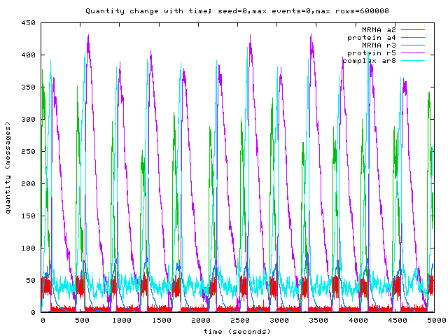
We’ve been thinking about using a stochastic π-variant with a join operator. Having join available allows the expression of state machines to be much more direct than in a joinless stochastic π. We started modelling the lambda-switch to fit the model from this BioConcur paper, and saw that it seems more natural to attach the reaction rate to each individual join rather than to each channel as BioSPI does.

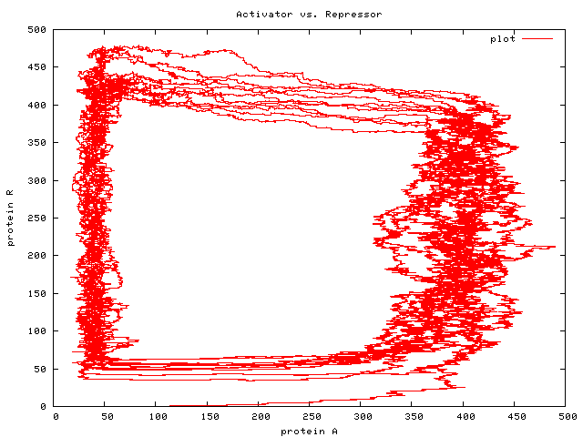
Bisimulation

The standard model has comm meaning interaction; we have comm meaning movement in some sense: atoms (mass) move from one locus (molecular species) to another, or a molecule undergoes conformational change, which is a kind of motion from one state or class or species to another. This means that bisimulation in the alternative model has to do with movement rather than interaction — which seems more fine-grained, but perhaps less natural.

Uncertainty in Biological Simulation

We also thought about a few properties biological simulation systems ought to have. One important one is a notion of uncertainty. Few of the current systems are honest about their limits — only one of the papers at BioConcur displayed error bars on any of its graphs! The systems in use all generate probable trajectories through state-space, and this is I assume implicitly to be understood by the reader of the various program outputs, but it would be useful to have the uncertainty in the results reflected in the various displays that these systems produce.

Besides the uncertainties that come from stochastic modelling and Monte-Carlo-type approaches in general, all the inputs to the systems (eg. rates) are purely empirical data, with associated uncertainties, and these uncertainties are not propagated through the system. Not only do the outputs not show the variation in results due to random sampling, but the outputs do not explore the limits of the accuracy of the inputs, either.

Reagent concentration vs. Gillespie vs. Modelling reagent state

The alternative model deals well with high reagent concentrations, since a high concentration is modelled as a large number of messages outstanding on a channel. The Gillespie scheduling algorithms are O(n)-time in the number of enabled reactions, not in the concentrations of the reagents. The standard model suffers here because each molecule is modelled as a process — that is, as an enabled reaction. In a naïve implementation, this makes the scheduling complexity O(n)-time (or at best, O(log(n)) time if the Gibson-Bruck algorithm is used) in the number of molecules in the system.

However, modelling molecules as processes seems to provide one advantage that doesn’t easily carry over into the alternative model: molecule-processes can involve internal state that any interacting molecule need not be concerned with. For example, enzyme-private channels with different rates associated with them might be used to model the different reactivities of phosphorylated and unphosphorylated states of the enzyme.

Perhaps a hybrid of the two models will be workable; after all, even in the alternative model, you have the freedom of the restriction operator available for implementing complex behaviours. The alternative model allows some common patterns to be expressed more simply than the standard joinless model though, it seems.

We’re still thinking about ways of keeping the molecules-as-messages approach while allowing reactions to specialise on molecule-message state or to ignore it, as appropriate.

Compartments

BioSPI 3.0 took the standard stochastic-π implementation and added BioAmbients to it (see the 2003 paper by Regev, Panina, Silverman, Cardelli and Shapiro). Any stochastic-join will probably benefit from being able to model compartments similarly.

The simple, ambientless approach suffers some of the same problems as SBML is facing with regard to recognising the similarity of species across compartments. Some way of factoring out reactions/processes/etc common across all compartments should be useful.

Last week I was privileged to be able to attend some of the workshops associated with Concur 2004, a conference on Concurrency Theory. Thanks, LShift!

• On the Monday I attended BioConcur ‘04. You can find my notes under category bioconcur.

• On the Saturday I attended AVoCS ‘04. My notes are under category avocs.

(Don’t forget that, blog-style, the most recent posts are at the top, so the notes should be read upward from the bottom of each page.)

The BioConcur talks really provided some food for thought. I’m looking forward over the next few months letting some of the ideas from the conference take root, and I’ll be tracking some of the various projects with interest. It’s an exciting time to be in systems biology.

(I also caught a bit of the previous talk on semantic subtyping for π. It looks great! Also very codenameesque… anyway, to the talk at hand:)

WWW is the application considered - probabilities of event occurrences are important there (probability of, what, packet loss? server error?), as in bioambients.

The exponential distribution function is 1-e^-rt

• if you use the exp. dist. fn, you have a CTMC
• and it’s memoryless

Ambients get decorated with a parameter η which is a scaling factor, controlling the rate of reaction inside the ambient. Also actions in, out etc. get decorated with a rate just like stochastic-π.

[How does that work with bioambients? Would the η be like volume there? What happens if you try to stuff a huge ambient inside a tiny one (in bio)?]

There’s no implementation yet. This is still very preliminary work.

Precise model-checking of models with continuous state variables is difficult. DTMCs and CTMCs, discrete and continuous time Markov Chains respectively, while able to optionally model continuous time cannot model a continuous state space, having only a discrete state space. (cf. PEPA) Markovian Reward Models have a strongly limited capability for modelling continuous state — limitations include for instance that the behaviour may not depend on the continuous state variable!

Stochastic Fluid Models do better [could it be applied to the RKIP/ERK pathway problem?] at the expense of significantly more difficult analysis. Only a very small number of continuous state variable can be handled.

I missed the end — had to leave to see the stochastic-ambients talk.

This talk was about using CSP within the Balsa toolkit to model asynchronous (clock-free) hardware. Asynchronous hardware replaces the clock with explicit synchronisation using handshakes/request + acknowledgement signals.

Clockless architectures are more efficient, cheaper in transistors, and they give more opportunity for verification. They’re harder to design and designs tend to be error-prone, though. This work is focussed on the idea that verification ought to be able to offset the difficulties of working with asynchronous systems.

At sub-micron technologies, the gates are so small the manufacturing process can be inaccurate enough to cause significant differences in timing delays within the chip! Hence per-chip clock-rate limits and testing… :-/

They’re compiling a CSPish language into silicon! Cool!

• syntax-directed compilation
• doesn’t pull extra parallelism out of the code
• so writing the parallelism in is very important
• which motivates the choice of CSP

CSPish language –> “handshake network” –> gate-level network –> …

Balsa has until now been a simulation-only tool, with no verification tool available. This work is building one.

• Each interface between handshake-network components has a more-or-less session type

• Different properties are verified at different levels - some at the whole-program balsa/csp level, some at the handshake-net level, and some at the gate network level

• the top levels are synchronous models (ie. output has a continuation); lower levels are async however! so new approach used to verify async variants of csp: “protocol-based closed-circuit testing” – reminds me of behavioural type system zipper checkers! (you supply the environment and make sure it goes to zero…)

• the case study reproduced a deadlock seen in the balsa simulator, and showed positively that the fix for the problem genuinely did remove the possibility of deadlock.

• protocol at gate level is a subset of the traces of the gate net — because they have to cope with async sends at that level (?)

• standard csp semantics, standard csp model-checkers. that is the contribution - no special tools required cf. Dill and cf. Josephs

The work is using BSPA - CCS for BSP - “Bulk synchronous process algebra”. BSPA is bilevel - local level and global level. The programmer can address processors by number within a machine, but can also send messages between machines.

There are two kinds of comm: computation within the par step; and also message-sending for the global transfer step and synchronisation barrier.

The cost model is to expand individual expression to serial form (by expanding par into sum-of-sequence) and from there using “cost rules” to arrive at an expression representing the cost of the calculation. The clever step is the recognition of the semi-ring (?).

• how is she locating the barrier expressions? sync trees?

• future work: use the cost model to evaluate the need for parallel processing, whether it would help or not in specific circumstances

This talk was about a particular graph language used to describe concurrent systems. The work focussed on analysing the graphs to identify symmetry in their Kripke structures, so that the symmetry could be reduced, thereby making the model more tractable.

Notes:

• using Promela to construct models

• is constructing the entire Kripke structure the expensive bit?

• processes and channels are typed; processes and channels are coloured by type in the diagrams

• only need to consider static topology, because if there’s symmetry in the static case, then all instances of the symmetry will introduce the same patterns of new channels later on

• “automorphism group”?

Time Petri Nets introduce timing constraints on normal Petri Nets — not sharp constraints, intervals are given for each constraint.

• “boundedness” for TPNs undecidable
• “reachability” for bounded petri nets decidable
• SCG = ??
• region graph = ??
• untimed CTL* = ??
• reachability + time CTL model-checking is decidable (1994)
• so: talk on relation between the two models
• aim: structural translation; correctness proof — both achieved
• the translation permits use of existing efficient tools for analysing TAs, eg. uppaal

Future work: real case studies, perhaps with uppaal — and investigate expressiveness — can TAs be translated back to TPNs?